Quick Start: Tutorial

In this 10-minute tutorial, we will solve the equation of a mass-spring-damper system using vip-ivp. Then, we'll demonstrate the event system by counting the number of oscillations.

Problem Statement

We consider a classic second-order mechanical system: a mass attached to a spring and a damper. The motion of the mass is governed by the differential equation:

$$m \ddot{x} + c \dot{x} + kx = 0$$

Where:

• $x$ is the displacement,
• $m$ is the mass,
• $c$ is the damping coefficient,
• $k$ is the spring constant.

We want to:

1. Simulate the motion of the system over time.
2. Count how many times the mass crosses the equilibrium point (i.e., $x = 0$).

Step-by-step

1. Define the parameters

import vip_ivp as vip

m = 1.0  # Mass (kg)
k = 10.0  # Spring constant (N/m)
c = 0.5  # Damping coefficient (N·s/m)

x0 = 1.0  # Initial position (m)
v0 = 0.0  # Initial velocity (m/s)

2. Build the system

Ordinary Differential Equations are inherently circular, as higher-order derivatives depend on variables that are themselves computed by integrating those derivatives. To manage this circular dependency, vip-ivp introduces the loop_node() function. A Loop Node acts as a placeholder for a variable whose definition will be completed later

To solve an ODE, follow these steps:

1. Create a loop node for the highest-order derivative of the equation. In our case: the acceleration $\ddot{x}$.
2. Integrate to obtain lower-order derivatives. In our case: the velocity $\dot{x}$ and displacement $x$.
3. Loop into the equation. In our case, $\ddot{x} =-\frac{1}{m}( c \dot{x} + kx)$.

a = vip.loop_node()  # Acceleration
v = vip.integrate(a, v0)  # Velocity
x = vip.integrate(v, x0)  # Displacement
a.loop_into(-(c * v + k * x) / m)  # Set acceleration value

3. Add an event

An event is a condition that triggers a specific action during the simulation. In the context of dynamical systems, the condition typically involves a variable crossing a threshold — for example, when a position variable crosses zero.

In this example, we want to create a counter that is incremented every time the position crosses zero. The condition is the zero-crossing, and the action is incrementing the counter.

3.1. Detect crossings

To create a variable that detects crossings, use the .crosses(value) method:

zero_crossing = x.crosses(0)

You can specify the crossing direction with one of:

• "rising" – when the variable crosses upward (e.g., from negative to positive),
• "falling" – when it crosses downward,
• "both" – triggers in either direction.

3.2. Creating the Counter

Let's create a Counter object that can be incremented:

class Counter:
    def __init__(self):
        self.count = 0

    def increment(self):
        self.count += 1
        print(f"Counter incremented to {self.count}")


counter = Counter()

3.3. Create the event

The crossing is the condition of the event, and the action is counter.increment().

To create the event, use the execute_on() function:

increment_event = vip.execute_on(zero_crossing, counter.increment)

The execute_on() function enables the creation of events that triggers user-defined functions.

4. Plot and solve

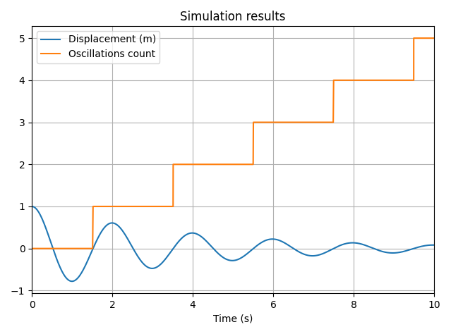
For quick visualization, variables can be marked for plotting using the .to_plot() method. When vip.solve() is called, all variables marked this way will be displayed in an automatically generated plot.

You can assign a label to each curve by passing a string to .to_plot() — this will be used as the legend in the plot.

# Choose results to plot
x.to_plot("Displacement (m)")
# Solve the system
vip.solve(10, time_step=0.01)

After solving, a plot window will open showing the selected variables over time.

5. Post-processing

After the system has been solved, you can access the simulation results directly from the variables.

Accessing variable values

Each variable has a .values property, which returns a NumPy array of its value over time. All variables also have a .t property, which holds the corresponding time values.

This makes it easy to use your favorite Python libraries (like matplotlib, plotly, or pandas) for advanced analysis or custom plotting.

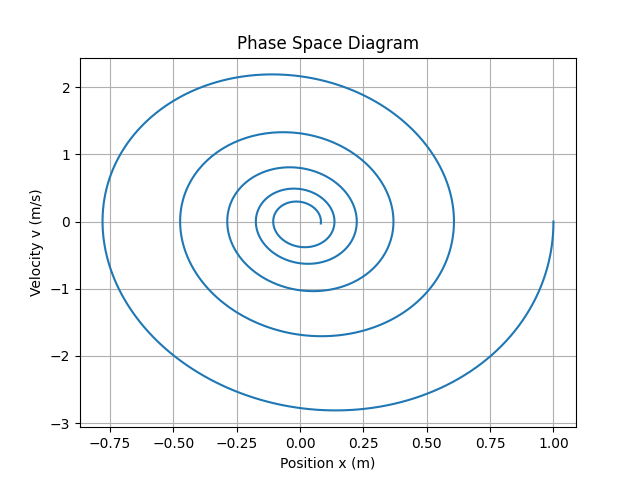
Here’s an example that creates a phase space diagram (position vs. velocity):

import matplotlib.pyplot as plt

# Create a phase space diagram
plt.plot(x.values, v.values)
plt.xlabel('Position x (m)')
plt.ylabel('Velocity v (m/s)')
plt.title('Phase Space Diagram')
plt.grid()
plt.show()

You’re free to combine vip-ivp with any Python tool for post-processing, making it a powerful and flexible option for simulation workflows.

Exporting the results

vip-ivp provides utilities to easily export simulation results for further analysis or storage.

• Use vip.export_to_df() to export one or more variables to a Pandas DataFrame.
• Use vip.export_to_file() to export directly to a CSV file.

Here’s an example that exports all the temporal variables to a DataFrame:

# Export the results to pandas
dataframe = vip.export_to_df()
print(dataframe)

The console prints the following results:

      Time (s)         v         x
0         0.00  0.000000  1.000000
1         0.01 -0.099734  0.999501
2         0.02 -0.198871  0.998007
3         0.03 -0.297316  0.995526
4         0.04 -0.394974  0.992064
...        ...       ...       ...
1006      9.96  0.002948  0.082447
1007      9.97 -0.005291  0.082435
1008      9.98 -0.013484  0.082340
1009      9.99 -0.021622  0.082164
1010     10.00 -0.029698  0.081907

[1011 rows x 3 columns]

Each row of the DataFrame corresponds to a time step, and columns include the time and the values of the selected variables.

You may notice that the number of rows is slightly higher than expected. For instance, if you simulate for 10 seconds with a time step of 0.01s, you might expect 1001 values — but the DataFrame shows 1006.

This is because vip-ivp automatically adds the exact times at which events occur, even if they fall between regular time steps. In the example, 5 crossing events were detected and added to the timeline, bringing the total to

If you prefer to keep a uniform time grid and exclude event times, you can pass the following option to solve():

vip.solve(10, time_step=0.01, include_crossing_times=False)

Complete example

import vip_ivp as vip
import matplotlib.pyplot as plt


class Counter:
    def __init__(self):
        self.count = 0

    def increment(self):
        self.count += 1
        print(f"Counter incremented to {self.count}")


counter = Counter()

# System parameters
m = 1.0  # Mass (kg)
k = 10.0  # Spring constant (N/m)
c = 0.5  # Damping coefficient (N·s/m)

x0 = 1.0  # Initial position (m)
v0 = 0.0  # Initial velocity (m/s)

# Build the system
a = vip.loop_node()  # Acceleration
v = vip.integrate(a, v0)  # Velocity
x = vip.integrate(v, x0)  # Displacement
a.loop_into(-(c * v + k * x) / m)  # Set acceleration value

# Create event that triggers when x crosses 0
zero_crossing = x.crosses(0)
increment_event = vip.execute_on(zero_crossing, counter.increment)

# Choose results to plot
x.to_plot("Displacement (m)")
# Solve the system
vip.solve(10, time_step=0.01)

# Create a phase space diagram
plt.plot(x.values, v.values)
plt.xlabel('Position x (m)')
plt.ylabel('Velocity v (m/s)')
plt.title('Phase Space Diagram')
plt.grid()
plt.show()

# Export the results to pandas
dataframe = vip.export_to_df(v, x)
print(dataframe)

Using Jupyter Notebook

Jupyter Notebook Compatibility

vip-ivp works seamlessly with Jupyter Notebook, but to ensure correct behavior, especially when re-running cells, you must initialize a new system before creating any TemporalVar instances:

import vip_ivp as vip

vip.new_system()

This line resets the internal state of the solver and avoids unintentional accumulation of old variables from previous runs.

warning

Always rerun vip.new_system() before creating Temporal Variables if you're re-executing a notebook cell.
Failing to do so will cause the simulation graph to grow with each run, which can **drastically slow down solving times **.

Complete example in a Notebook

Bouncing ball example in a Notebook